The Slippage Ratio: A New Metric to Understand Curve.fi’s AMM Protocol

The Curve Whitepaper concisely highlights an approach to building an AMM that allows developers to control slippage. Curve’s primary use case is swapping stablecoins, where low slippage is essential to compete with centralized exchanges. In contrast, Uniswap and Balancer use a constant-product invariant (as the Curve Whitepaper describes it); on Uniswap, slippage would be 25% for a trade that is 10% of the size of a liquidity pool. Intuitively, this isn’t acceptable for two assets that are nominally equivalent e.g., USDC vs DAI.

Curve.fi has maintained a large and stable market share, indicating the success of its approach (see figure 1). It’s natural to consider whether the protocol might be applicable to any token pair that has a notion of parity. By parity, I mean that there is some kind of “normal” or mean-reverting price implicit in the asset. For example, a corporate bond issued by General Motors would be expected to trade around 1.0 (i.e., par), barring some kind of credit or interest rate event. We can characterize GM-bond/USD as a parity token pair. A stablecoin is just one example of a parity token pair.

Figure 1. Weekly DEX Volume Market Share

The rest of this post considers the Curve AMM protocol (also called the StableSwap Invariant in the Whitepaper) in the context of any parity token pair. Stablecoins are expected to always trade at or near 1.0; in general, however, the price of a parity token pair may deviate substantially from 1.0. Therefore, we have to give serious consideration to the protocol’s stability in such scenarios. In doing so, I introduce the slippage ratio, which measures the slippage of an AMM protocol at a given pair price. For the Uniswap AMM, the slippage ratio is always 2. But for Curve.fi, the slippage ratio is dependent on the pair price.

Defining the Slippage Ratio

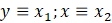
Let x and y be the quantities of two pairs in a liquidity pool. For example, y might be the quantity of USDC and x might be the quantity of another parity token (e.g., a 3-year USDC denominated loan collateralized by WBTC). By definition,

If Δx is small, then there is 0 slippage and we can write

Assuming there are no arbitrage opportunities, we can assume that the zero-slippage price is exogenous. Let π be the exogenous market price of a pair. In a no-arbitrage equilibrium, the pair price is defined by

An AMM protocol is defined by a functional relationship between x and y i.e.,

We can write out f(x) as a Taylor Series expansion i.e.,

Therefore,

Now we can define slippage as follows

In general, slippage will vary based on the size of a trade relative to a liquidity pool’s size. Therefore, it’s natural to normalize the slippage by the trade size.

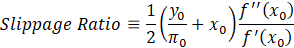
Now we can define

This quantity characterizes the slippage for a trade that is “small” relative to the liquidity pool’s market value.

The Constant-Product Invariant a.k.a., Uniswap

I’ll first consider the slippage ratio for a constant-product invariant AMM (e.g., Uniswap).

Taking the first derivative, we have

Therefore,

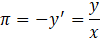
In other words, the market price is equal to the ratio of the quantities of the two pairs. Note that this result is unique to a constant-product invariant. It is not a general feature of all AMM protocols. Moreover,

Therefore,

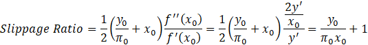
But note that

Therefore,

In other words, a trade that is 1% of the liquidity pool’s size would have slippage of ~2%. (The actual slippage for a 1% trade is 2.04%.)

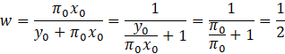
Finally, token two’s market value weight is

We now have three unique properties of a constant-product invariant:

1) The market price is always equal to the ratio of the quantities of the two tokens

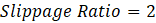
2) The slippage ratio is always 2

3) The market value weights remain constant (50/50 in the case of Uniswap)

The StableSwap Invariant a.k.a., Curve.fi

The Curve Whitepaper describes the StableSwap invariant in terms of n coins (with equal weight) in a single liquidity pool.

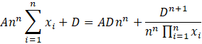
D is the variable that remains constant before and after a given trade.

A is called an amplification coefficient in the Curve Whitepaper. This subjective parameter is set based on the desired properties of the AMM. For example, a higher value of A would decrease slippage (at least at certain price points).

If n=2,

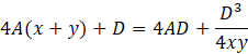
where

To understand this formula better, let A=0. Then

which of course is the constant-product invariant. If we write y=f(x), note that

and

In other words, when x=y, the zero-slippage price is exactly 1.

On the other hand, as A approaches infinity, we have

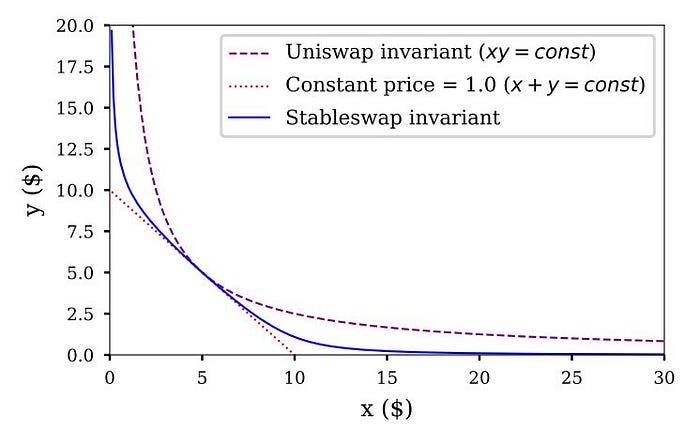
which is what the Curve Whitepaper calls a linear invariant or a constant-sum invariant i.e., the case where the two coins always have the same price.

As before, we have

and

Again, when x=y, the price is 1. In other words, the constant-sum and constant-product invariants are similar when the stablecoin pair has equal quantities in the liquidity pool. Figure 2 shows the StableSwap invariant relative to these two special cases.

Figure 2

In order to implement this algorithm, one has to solve for D. The Curve Whitepaper considers any number of coins i.e., we have to solve an n-degree polynomial. If n>3, there is no closed-form solution. Hence, Curve.fi apparently solves for D numerically. Here’s the relevant snippet from Github.

But since we’re focusing on a pool with just 2 pairs, we can derive a closed-form solution.

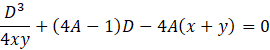
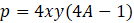
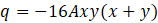
Using Cardano’s formula for a cubic polynomial, we have

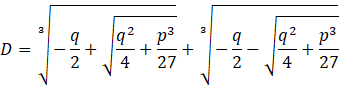
where

To implement this protocol, we also need to solve for y.

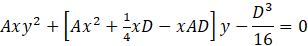
Using the quadratic formula, we have

As discussed earlier, the zero-slippage price of the pair is determined by the first derivative of this curve i.e.,

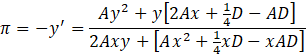
Moreover, as before,

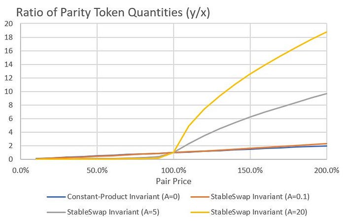
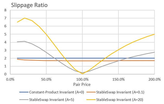
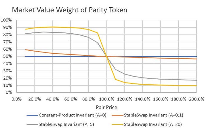
We can use the above formulae to evaluate how the StableSwap invariant behaves at various price levels. The results are shown in figures 3, 4, and 5. Note that the x-axis in all these graphs is the exogenously determined pair price.

Figure 3

Figure 4

Figure 5

Conclusions

The StableSwap AMM has clear advantages over the constant-product invariant:

1. It’s flexible i.e., the constant-product invariant is a special case of the StableSwap invariant
2. It enables a dramatic reduction in slippage under normal circumstances i.e., when the price is close to par
3. It’s inherently stabilizing. In order to drive prices below par, traders would have to actively sell the parity token into the AMM. For example, when A=20, 85% of the liquidity pool has to consist of the parity token to drive prices down to 80%.

However, the StableSwap AMM also has some cons:

1. The slippage can be much higher than a constant-product invariant if the pair price deviates significantly from par
2. As mentioned above, the market value weights need to vary in order to drive prices above or below par. This means that larger trades need to be executed in order to maintain a no-arbitrage equilibrium. As fewer players are able to trade in larger sizes, the StableSwap AMM might be prone to longer-lasting market dislocations. In other words, the AMM price might deviate from off-chain prices for a longer period of time.

References

https://en.wikipedia.org/wiki/Quadratic_formula

Cardano formula

DEX metrics 📊

https://github.com/curvefi/curve-contract/blob/master/contracts/pools/usdt/StableSwapUSDT.vy